2D Hord 296-B Tutorial

This tutorial will cover the basics of setting up and running the fluid problem of a cavitating flow over a hydrofoil. Additionally, a comparison of Loci-Stream results will be presented. Files for running the case yourself can be found HERE.

This example problem is based on the Hord cavitation experiments performed in the 1970s. The Hord experimental data is used to validate cavitation models because it is one of the few empirical studies with the reported data from instrumentation that can be easily replicated in simulation. The 296-B hydrofoil case was used for this example. The flow is cryogenic nitrogen that passes over a hydrofoil as it sits in a closed channel. The reduction in area for the flow to move as it encounters the hydrofoil results in a drop in the pressure, and the pressure falls below the saturation vapor of the nitrogen. This results in a bubble of nitrogen vapor forming and attaching itself to the leading edge of the hydrofoil. For reference, the paper containing the experimental data is: Cavitation in Liquid Cryogens II-Hydrofoil, Hord, NASA. The files that are needed to run this case can be extracted from a gzipped archive located here. The files will extract into a directory structure that mirrors this case’s location in the tutorials repository.

Geometry and Boundary Conditions

The geometry and boundary conditions for this case are shown below. In this case a flow of liquid nitrogen enters the domain from the left boundary and flows to the right across the hydrofoil. All no-slip walls are specified as adiabatic boundaries. A fixed-pressure outlet type is specified at the right boundary.

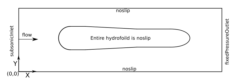
Geometry and boundary conditions for the Hord 296-B tutorial.

Grid

A mixed triangular/quadrilateral cell grid was first generated using SolidMesh. This was then extruded by SolidMesh into a single-cell thick grid in the z-direction. The grid is comprised of 144,552 prismatic/hexahedral cells. Particular emphasis during the grid-generation phase was place on proper resolution of the wall boundary layers, and extra resolution was placed around the upper leading region of the hydrofoil as that is where a vapor bubble forms. A few images of select regions of the grid are shown below.

A view of the grid around the hydrofoil.

Zoomed view of the grid around the upper leading edge of the hydrofoil.

Run Control File Setup

The run control file for the simulation is shown below.

Run control file for the case.

// Load the cavitation module.
loadModule: cavitation_nist
{

// Case 296-B:
// T0=88.54 K, P0=657484 Pa, Pv=316814 Pa, v0=23.7 m/s, rho0=753.8 kg/m^3
// Cavitation number = 2*(P0-Pv)/(rho*v0*v0) = 1.61
// Flow over time = (2.5 in)*(0.0254m / 1 ) / 23.7 m/s = 0.00268 s

// Turbulence notes:
// v0=23.7,L=D=0.0254*0.312=7.9248e-03,omega=10*v0/L=30284.7,nu=1.5886e-04/804.79,nut=nu,k=nut*omega=5.98e-03

// Note: The back pressure is set to 650000 in order to get P0 on the centerline at the inlet.

// Grid file information
grid_file_info: <file_type=VOG, Lref=1m, pieSlice>

boundary_conditions:
<
 TopSurface=noslip(adiabatic),
 BottomSurface=noslip(adiabatic),
 BackSurface=noslip(adiabatic),
 Inlet=subsonicInlet(v=23.7 m/s, T=88.54 K, k=5.98e-03, omega=30284.7, vapor_y=0.0, NCG_y=0.0),
 Outlet=fixedPressureOutlet(p=650000 Pa),
 TopBoundary=noslip(adiabatic),
 BottomBoundary=noslip(adiabatic),
 BC_11=symmetry,
 BC_12=symmetry
>

// Initial condition
initialCondition: <vapor_y=0.0, NCG_y=0.0, v=0.0 m/s, p=650000.0 Pa, T=88.54 K, k=5.98e-03, omega=30284.7>

// Flow properties
flowRegime: turbulent
flowCompressibility: compressible

// Equation of state and transport properties
// Using tabulated NIST EOS.
liquid_model: NITROGEN
vapor_model: NITROGEN
transport_model: module

// Time-stepping
timeIntegrator: BDF
timeStep: 1.0e-04
numTimeSteps: 4001
convergenceTolerance: 1.0e-19
maxIterationsPerTimeStep: 1

// Inviscid flux
inviscidFlux: SOU
turbulenceInviscidFlux: SOU

// Gradient limiting
limiter: venkatakrishnan

// Linear solver options
linearSolverTolerance: 1.0e-03
hypreSolverName: GMRES

// Diagnostics variables
// turnoverTime: Used to normalize pResidualTT
diagnostics: <turnoverTimeScale=2.68e-03>

// Momentum equation
momentumEquationOptions: <linearSolver=SGS,relaxationFactor=0.7,maxIterations=5>

// Pressure equation
pressureCorrectionEquationOptions: <linearSolver=HYPRE,relaxationFactor=0.1,maxIterations=20>
  pressureCorrectionLHSCompressibleTerms: on
  pressureBasedMethod: SIMPLEC
  PclipMin: 30000.0
  PclipMax: 1500000.0

// Energy equation
energyEquationOptions: <linearSolver=SGS,relaxationFactor=0.7,maxIterations=5,form=temperature>
  TclipMin: 68.478  //From the .sat file
  TclipMax: 95.0

// Turbulence equation
turbulenceEquationOptions: <model=menterSST,linearSolver=SGS,relaxationFactor=0.7,maxIterations=5>
  kFreestream: 5.98e-03
  omegaFreestream: 30284.7
  eddyViscosityLimit: 1e6

// Cavitation equation
cavitationEquationOptions: <linearSolver=SGS,relaxationFactor=0.3,maxIterations=5,source=SauerSchnerr>
  SauerSchnerrSourceParameters: <RB=3.0e-06, n=4.8e8>
  cavitationInviscidFlux: SOU
  AlphaViscosity: 1.0e-4
  cavitation: on

  // Non-condensable gas specification
  nonCondensableGasProperties: <m=28.9647 g/mol,cp=1005 J/kg/K,mu=1.805e-5 kg/m/s,kcond=0.02476 W/m/K>  //Nitrogen

// Reference values
// Used for both residual normalization and cavitation source term.
referenceValue: <L=0.00792, rho=753.8, v=23.7, k=1.0, omega=1.0>

// Printing, plotting and restart parameters
print_freq: 100
plot_freq: 100
plot_output: pResidualTT, kconduct, cp, laminarViscosity, vapor_y, vapor_vof, liquid_y, liquid_vof
plot_modulo: 0
restart_freq: 1000
restart_modulo:0

// Probes
probe_freq: 1
probe: <
 inletCenterline=[-0.0986,0.0,0.0039624]
>

}

In the following, we briefly discuss some of the key choices made in setting the run control file parameters for this case.

1. In the grid_file_info variable, we have placed the pieSlice option, because we are solving a 2-D flow on the grid. This option causes Stream to zero out the velocity field in the z-coordinate direction for all computations. When using this option, it is important that the grid be oriented such that the extruded direction is the z-dimension.

Running the Simulation

In the tutorial main directory are three files that are required to run the case.

• case.vog: the grid

• case.vars: the run control file

• NITROGEN.liq: the NIST database file for liquid nitrogen, created by the cavitation tool provided with Stream

• NITROGEN.vap: the NIST database file for nitrogen vapor, created by the cavitation tool

• NITROGEN.sat: the NIST database file for nitrogen saturation, created by the cavitation tool

For this case, the grid has around 145,000 cells. Stream has parallel efficiency down to 5,000 cells per processor, so you will want to run using less than 30 processes for the value passed to the -np argument in the mpirun command shown below. Using fewer processes is fine and will only result in an increased time for the solution to be generated. Execute the code using the following command.

mpirun -np 30 <path_to_stream_exec> --scheduleoutput -q solution case >& run.log_0 &

The case will run until the number of timesteps specified in the case.vars file is reached. Restart checkpoint solutions will be written to the restart/ directory at the number of timesteps specified in the case.vars file for the restart_freq variable.

Results

The results from the simulation of the Hord hydrofoil case are compared to experimental data that was provided. Temperature and pressure data along the upper surface of the hydrofoil is plotted against the empirical data. The Schnerr-Sauer cavitation model was used. Stream also supports other models that are specified in the Stream user guide.

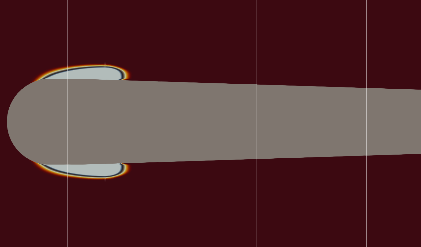
Locations of the pressure taps on the upper surface of the hydrofoil.

Shown in the image above are the x-coordinate stations that correspond to the locations where the data was measured in the Hord experiments. Below are pressure and temperature plots along the top surface of the hydrofoil.

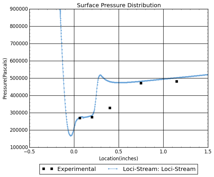
Pressure along the top surface of the hydrofoil.

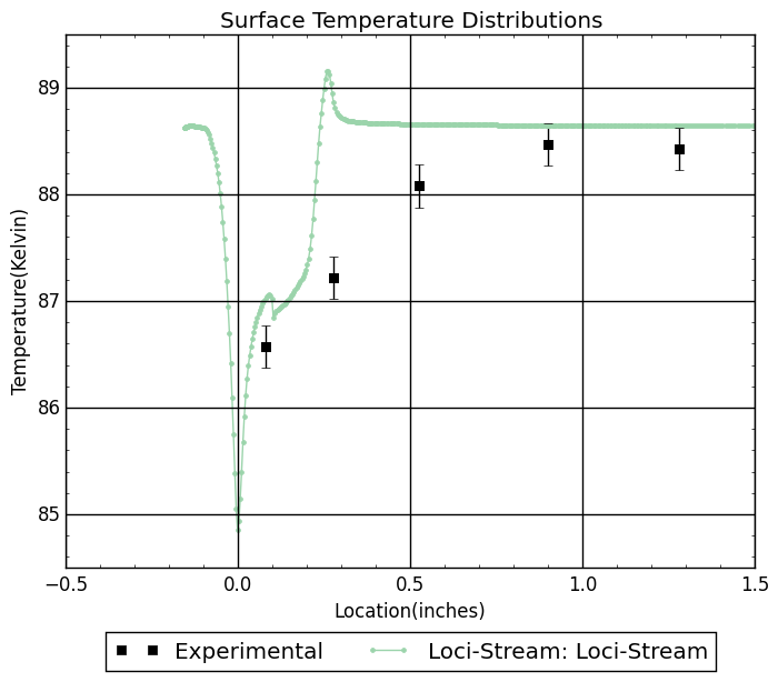
Temperature along the top surface of the hydrofoil.

The extract program is the utility that is used to view the results of a simulation. For this case we view the simulation at time step 4000. In the run directory extract the solution using: extract -vtk case 4000 P v vapor_y . This will generate a solution directory with files in the Paraview VTK format which can be opened by Paraview. 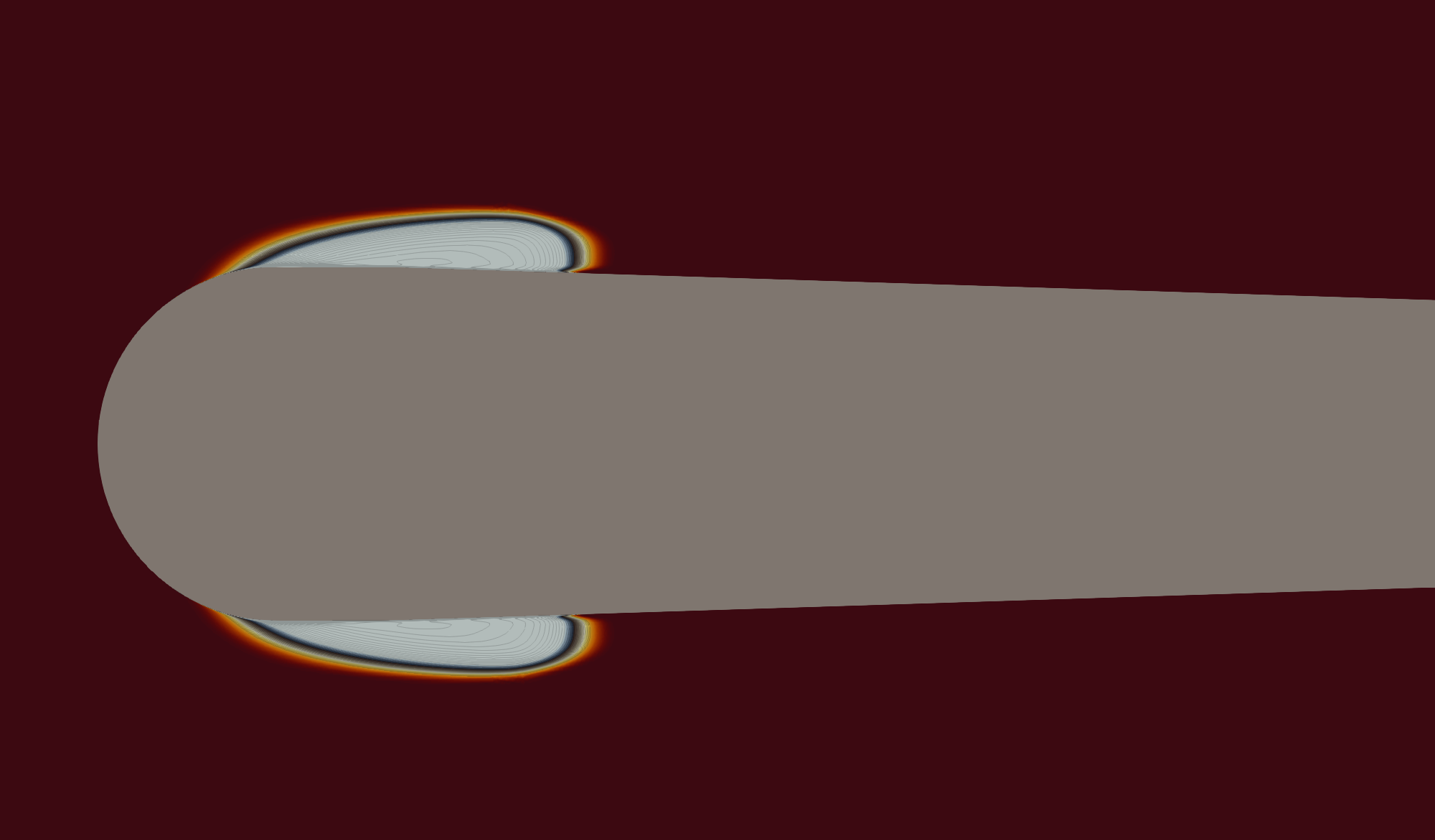The case name is case and the time step is 4000, and the variables to extract are the pressure(P), velocity(v), and vapor mass fraction(vapor_y). Below is a contour plot of the magnitude of the vapor mass fraction field, which was created using Paraview.

Contour plot of the magnitude of the vapor_y mass fraction field.