2D Cavity Flow Tutorial

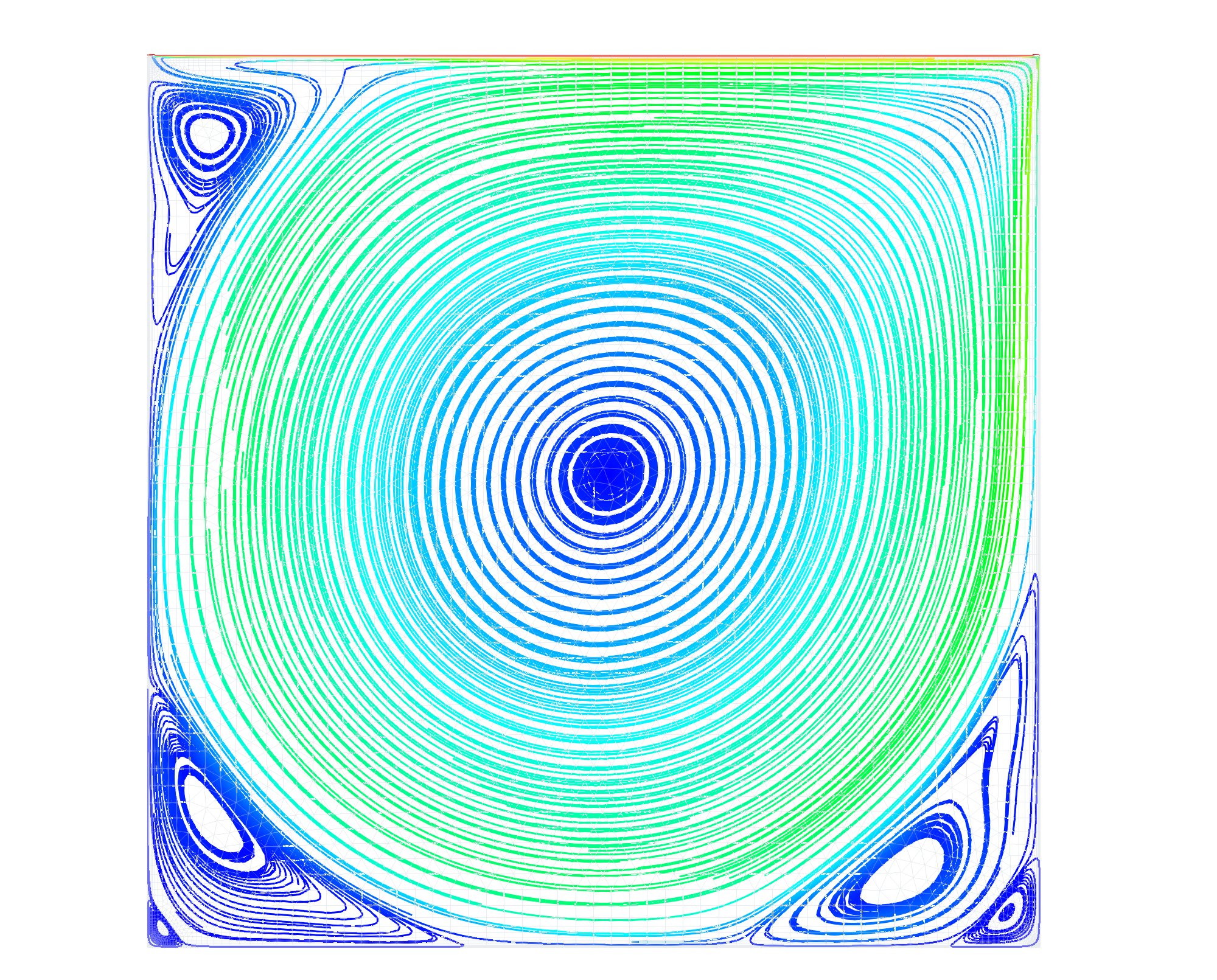
This tutorial will cover the basics of setting up and running the common fluid problem of the flow in a cavity. The cavity flow problem is a canonical problem in computational fluid dynamics (CFD). It is often given to students as a project in their first course on the topic of CFD. The flow is incompressible, viscous, and bounded within a sealed 2D box. The top of the domain moves to the right continuously, which drags the viscous fluid to the right. A steady-state flow pattern develops within the box after some time, which can be seen in the image above. The files that are needed to run this case can be extracted from a gzipped archive located here. The files will extract into a directory structure that mirrors this case’s location in the tutorials repository.

Geometry and Boundary Conditions

In this case, the domain is a 2D box with a moving top wall. The top wall moves to the right at a constant velocity. The walls do the domain are no-slip walls.

Diagram of the cavity flow problem.

Grid

A mixed triangular/quadrilateral cell grid was first generated using SolidMesh. This was then extruded by SolidMesh into a single-cell thick grid that is extruded in the z-direction. The grid is comprised of 11,725 prismatic cells. An image of the region near the particle is shown below.

Cavity flow domain grid

Run Control File Setup

The run control file for the simulation is shown below.

Run control file for the case.

{
// Grid file information
grid_file_info: <file_type=VOG, Lref=1m, pieSlice>


// Lid driven cavity flow example. The Reynolds number for this example is set to 500,
// which gives the following properties based on the definition of the Reynolds
// number: Re = rho*V*L/mu, with values of V=1 m/s, rho=1000 kg/m^3, L=0.1 m,
// and mu=1.0e-2 Pa*s. This gives a Reynolds number of 10000.
boundary_conditions: <
 Walls=noslip(),
 Top=incompressibleInlet(v=1 m/s),
 BackWall=symmetry(),
 Frontwall=symmetry()
>

// Initial conditions
initialCondition: <rho=1000, p=1 Pa, v=0.0m/s>

// Flow properties
flowRegime: laminar
flowCompressibility: incompressible

// Equation of state and transport properties
transport_model: const_viscosity
mu: 1.0e-2

// Time-stepping
timeIntegrator: BDF
timeStep: 1.0e+30
numTimeSteps: 10001
convergenceTolerance: 1.0e-30
maxIterationsPerTimeStep: 1

// Inviscid flux
inviscidFlux: SOU

// Gradient limiting
limiter: venkatakrishnan

// Linear solver options
linearSolverTolerance: 5.0e-02
hypreSolverName: AMG

// Set the turn-over time scale used to normalize residual turn-over time values.
diagnostics: <turnoverTimeScale=1.0e-1>

// Momentum equation
momentumEquationOptions: <linearSolver=SGS,relaxationFactor=0.7,maxIterations=3>

// Pressure equation
pressureCorrectionEquationOptions: <linearSolver=HYPRE,relaxationFactor=0.2,maxIterations=20>
  pressureBasedMethod: SIMPLEC

// Printing, plotting, and restart parameters
print_freq: 50
plot_freq: 500
plot_modulo: 0
plot_output: pResidualTT
restart_freq: 2000
restart_modulo: 0

}

Running the Simulation

In the tutorial main directory are three files that are required to run the case.

• case.vog: the grid

• case.vars: the run control file

For this case, the grid has around 12,000 cells. Stream has parallel efficiency down to 5,000 cells per processor, so you will want to run using less than 3 processes for the value passed to the -np argument in the mpirun command shown below. Using fewer processes is fine and will only result in an increased time for the solution to be generated. Execute the code using the following command.

mpirun -np 3 <path_to_stream_exec> --scheduleoutput -q solution case >& run.log_0 &

The case will run until the number of timesteps specified in the case.vars file is reached. Restart checkpoint solutions will be written to the restart/ directory at the number of timesteps specified in the case.vars file for the restart_freq variable.

Results

The extract utility is used to view the results of a simulation. For this case we view the simulation at the 10,000th time step. In the run directory extract the solution using the command: extract -vtk case 10000 P v . This will generate a solution directory with files in the Paraview VTK format which can be opened by Paraview. The case name is case and the time step is 10000, and the variables to extract are the pressure(P) and velocity(v).

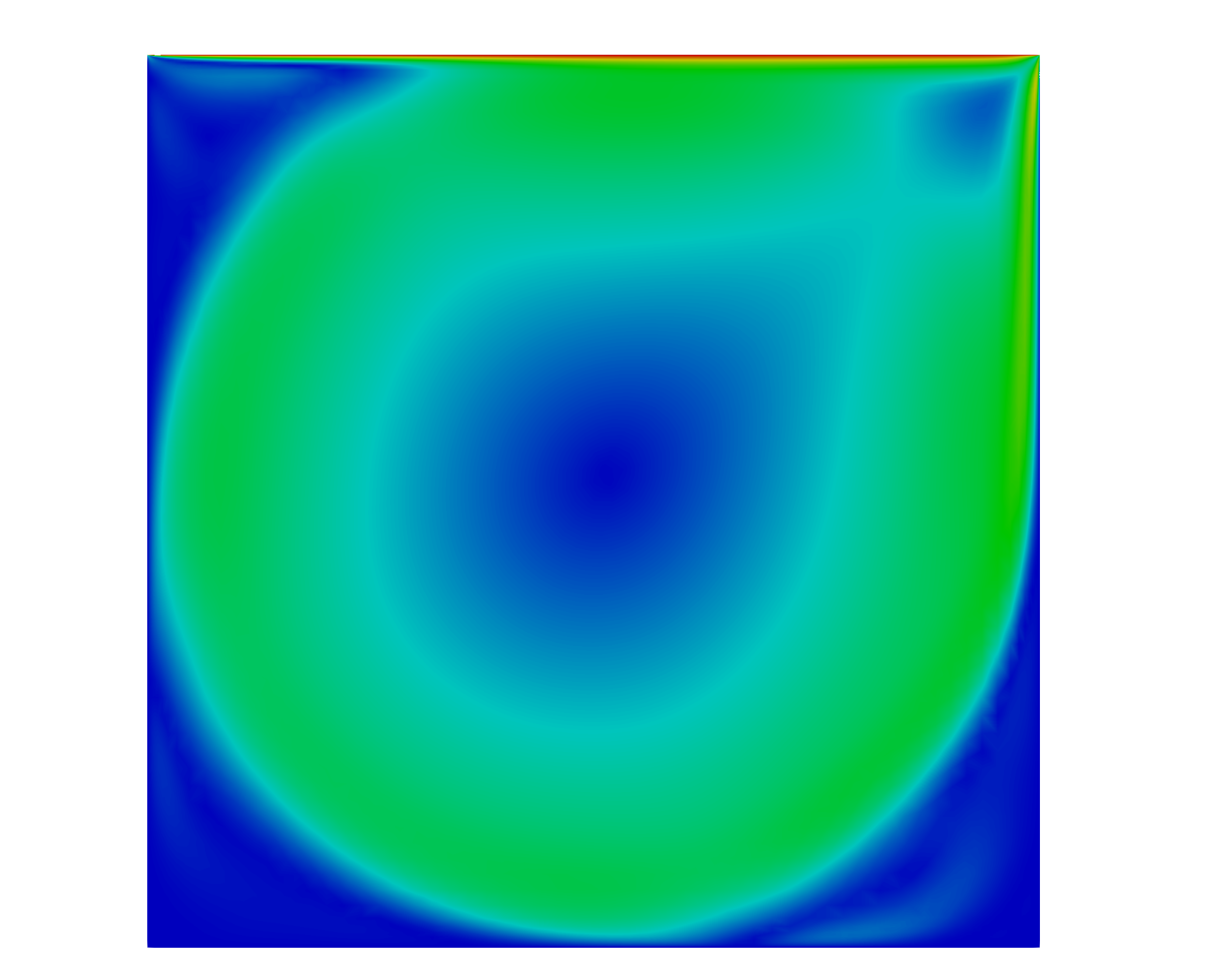
A contour plot of the velocity magnitude within the cavity

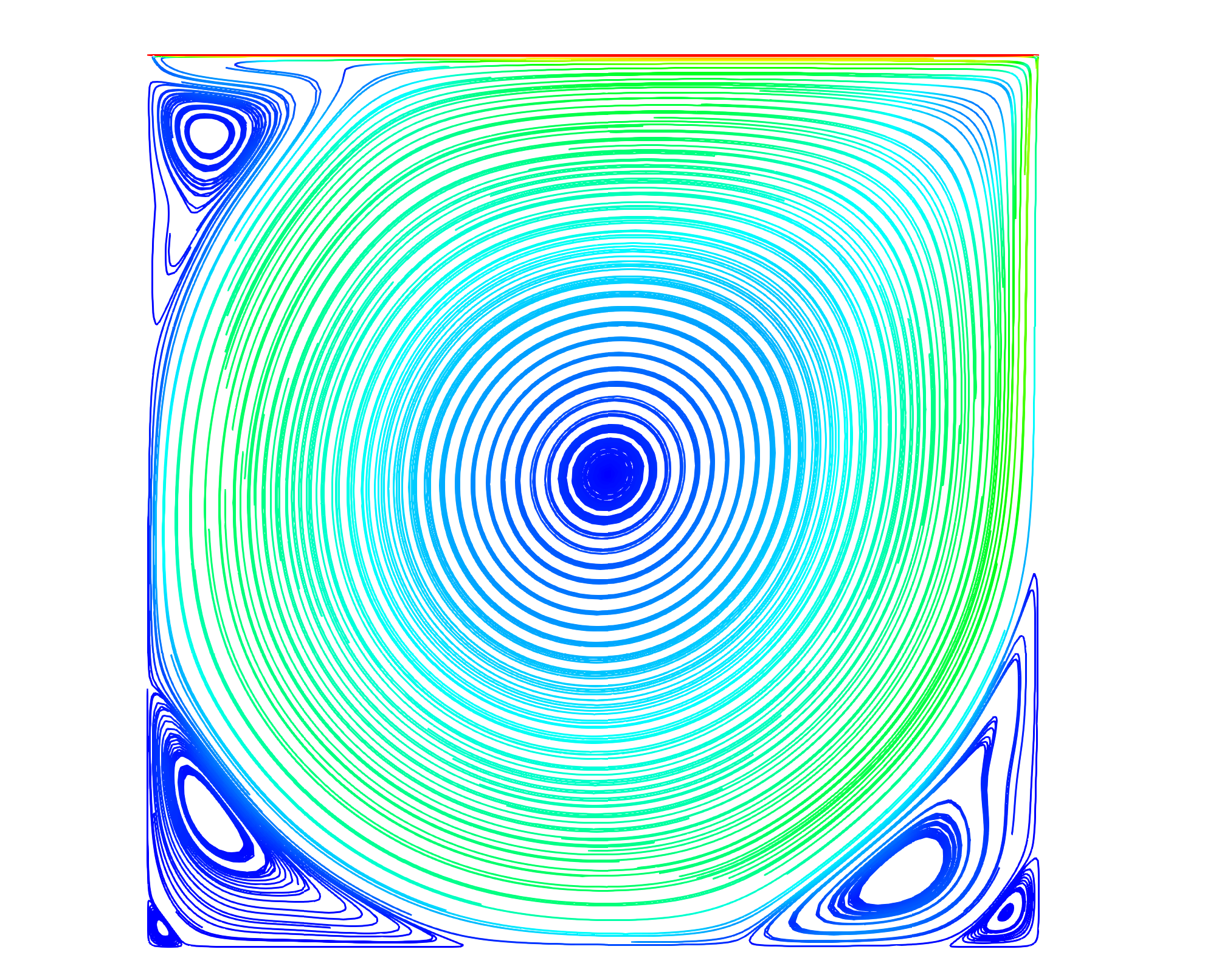
A stream-traced plot of the velocity field. A set of secondary vortices in the corners can be seen as well as the formation of tertiary vortices.