3D RCM-1 Flamelet Tutorial

This tutorial covers the basics of setting up and running the RCM-1 combustion test case, which is commonly used in the CFD community for testing combustion models for turbulence/chemistry interaction. In this example, we employ a 3-D grid and use RANS turbulence modeling to obtain a steady-state solution to the problem. This RANS solution can then used as an initial condition for an unsteady detached-eddy simulation (DES). The files that are needed to run this case can be extracted from a gzipped archive located here. The files will extract into a directory structure that mirrors this case’s location in the tutorials repository.

Geometry and Boundary Conditions

The geometry and boundary conditions for this case are shown below. Fuel, composed of 40.18% H2 and 59.82% H2O by mass, enters the domain through the outer annular inlet. Oxidizer, composed of 94.49% O2 and 5.51% H2O by mass, enters the domain through the central annular inlet. With the exception of the upper combustion chamber wall which has a specified temperature profile, all walls are specified as adiabatic boundaries. Flow at the nozzle exit becomes supersonic before steady state is achieved, and is specified as an extrapolated-pressure outlet for the duration of the simulation.

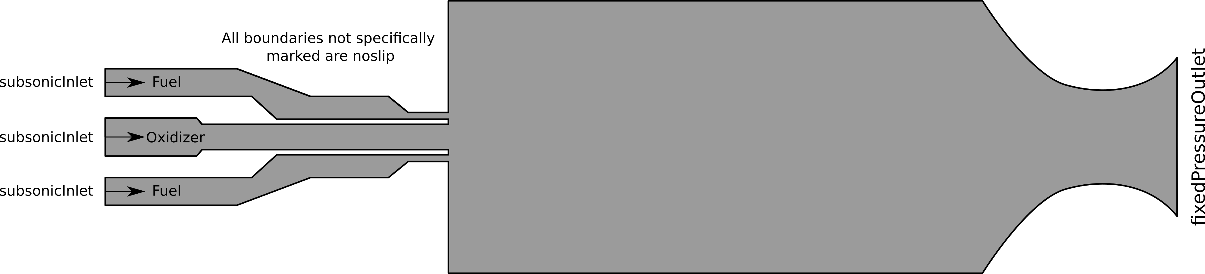
Geometry and boundary conditions.

Grid

A 3-D surface for the RCM-1 combustor was drawn using the OnShape CAD software. This IGES formatted surface description was loaded into the Capstone Create CAD/Meshing program and a surface mesh was generated. This surface mesh was then exported to a UGRID mesh format and then used as an input to the AFLR3D mesh generator, which resulted in a 3-D mesh comprising 6,844,905 prismatic/hexahedral cells. The inlet manifold section for this case has been shortened from the 2-D case in order to reduce the grid size for the purposes of this tutorial. Close-up images of select regions of the grid are shown below.

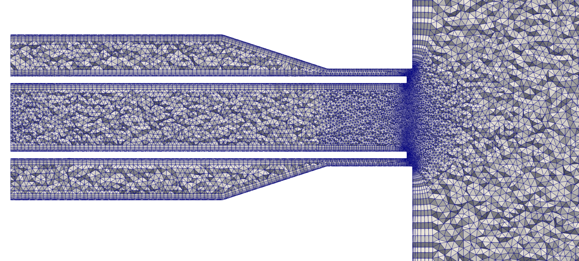
The upstream region of the grid.

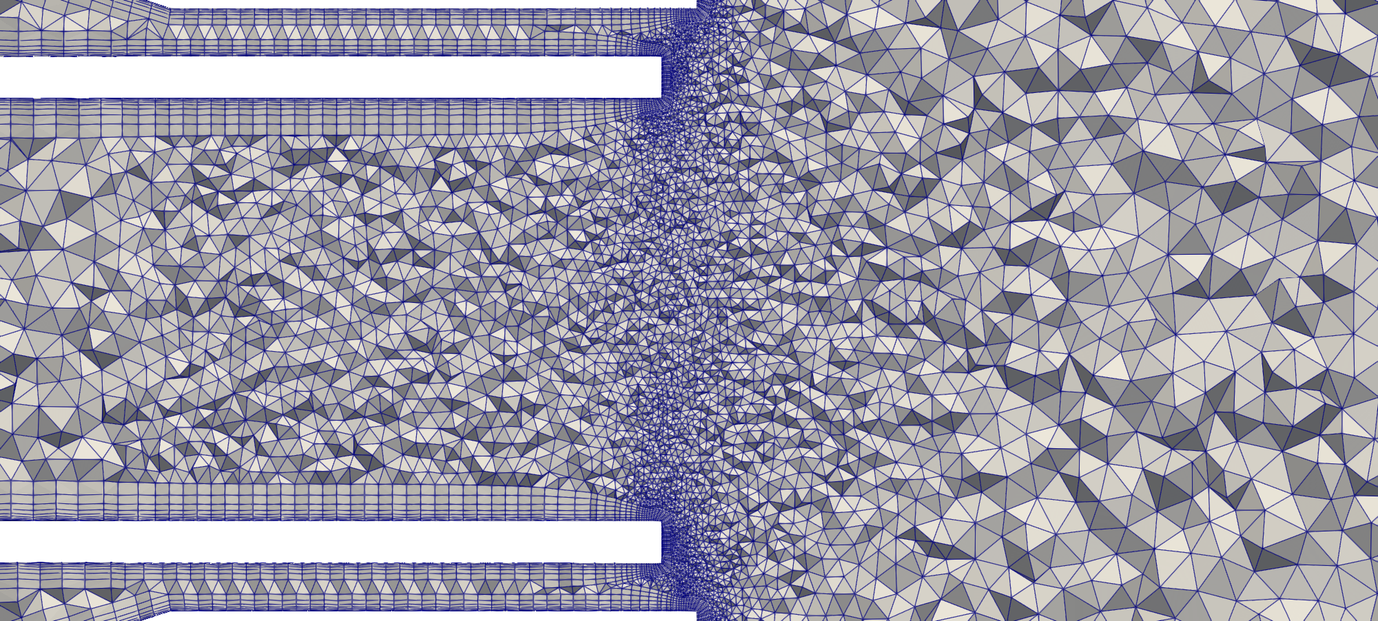
The combustion post region of the grid.

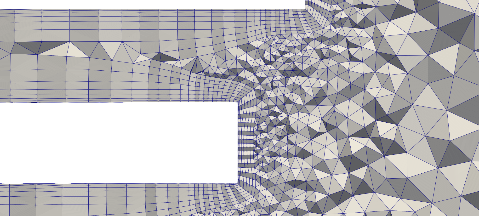
Zoomed view of the combustion post region of the grid.

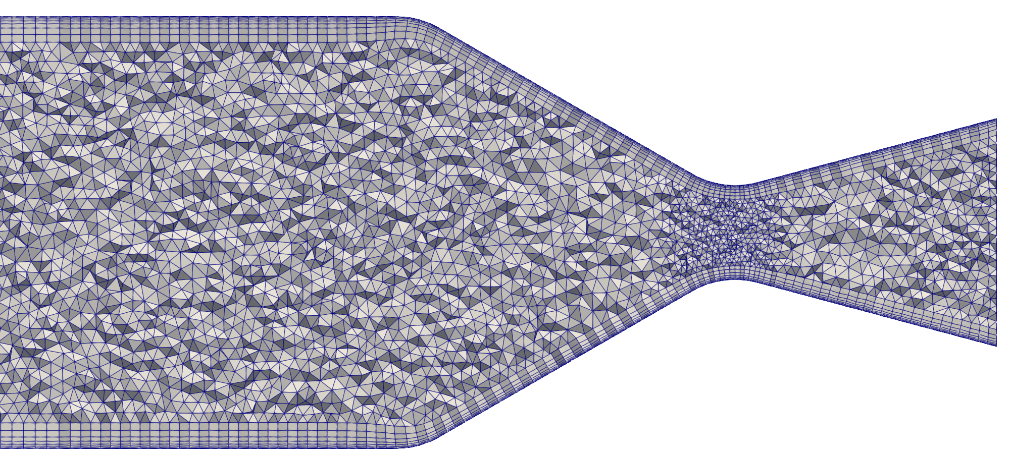
The nozzle region of the grid.

Run Control File Setup for RANS Simulation

The run control file for the RANS simulation is shown below.

Run control file for the RANS case.

// Load the compressible flamelet module
loadModule: compressible_flamelet_tf

{

// Grid file information
grid_file_info: <file_type=VOG,Lref=1 m >

// Boundary conditions
boundary_conditions:
<
 Fuel_inlet=subsonicInlet(mdot=3.33111993e-02 kg/s,T=800 K,Z=1.0,C=0.5982,k=4.2,omega=12900.0),
 Nozzle=noslip(adiabatic),
 ChamberWalls=noslip(adiabatic),
 Fuel_Walls=noslip(adiabatic),
 Oxidizer_Walls=noslip(adiabatic),
 Post_Tip=noslip(adiabatic),
 Face_Plate=noslip(adiabatic),
 Oxidizer_inlet=subsonicInlet(mdot=9.0447402E-02 kg/s,T=711 K,Z=0.0,C=0.0551,k=0.5,omega=37950.0),
 Outlet=extrapolatedPressureOutlet
>

// Initial condition
initialCondition: <v=[0.0 m/s,0.0 m/s,0.0 m/s],p=5.4e+06 Pa,T=3174.0 K,Z=0.34,C=0.912,k=0.5,omega=37950.0>

// Flow properties
flowRegime: turbulent
flowCompressibility: compressible

// Transport model set to 'module' since all properties gotten from flamelet table.
transport_model: module

// Time-integration parameters
timeIntegrator: BDF
timeStep: 5.0e-06
numTimeSteps: 10001
convergenceTolerance: 1.0e-12
maxIterationsPerTimeStep: 11

// Inviscid flux
inviscidFlux: FOU
turbulenceInviscidFlux: FOU
flameletInviscidFlux: FOU

// Gradient limiting
limiter: venkatakrishnan

// Linear solver options
linearSolverTolerance: 5.0e-03
hypreSolverName: AMG
hypreStrongThreshold: 0.9

// Diagnostics variables
//  turnoverTimeScale: used to normalize residual turn-over time (TT) values
diagnostics: <turnoverTimeScale=4.6e-03>

// Momentum equation
momentumEquationOptions: <linearSolver=SGS,relaxationFactor=0.3,maxIterations=5>

// Pressure correction equation
pressureCorrectionEquationOptions: <linearSolver=HYPRE,relaxationFactor=0.1,maxIterations=20>
  pressureBasedMethod: SIMPLEC
  PclipMin: 20000.0
  PclipMax: 20000000.0

// Energy equation
energyEquationOptions: <linearSolver=SGS,relaxationFactor=0.3,maxIterations=5,form=totalEnergy>
  TclipMin: 500.0
  TclipMax: 5000.0

// Turbulence equations
turbulenceEquationOptions: <model=menterSST2003,linearSolver=SGS,relaxationFactor=0.7,maxIterations=5>
  kFreestream: 4.2
  omegaFreestream: 12900
  eddyViscosityLimit: 10000

// Flamelet equations
flameletEquationOptions: <linearSolver=SGS,relaxationFactor=0.3,maxIterations=5>
  combustion: on

// Available combustion models
combustionModels:
<
  nonpremixed=flamelet(table="burke_fpvc_ideal_20200601.h5")
>

// Combustion model selection by region
combustionModelRegions:
<
  regions=[ inBox(p1=[-1.0e+30,-1.0e+30,-1.0e+30],p2=[1.0e+30,1.0e+30,1.0e+30],model=nonpremixed) ]
>

// Printing, plotting and restart parameters
print_freq: 1000
plot_freq: 1000
plot_modulo: 0
plot_output: ZZ,C,e,viscosityRatio
restart_freq: 1000
restart_modulo: 0

}

In the following, we briefly discuss some of the key choices made in setting the run control file parameters for this case.

1. The temperature profile for the ChamberWalls boundary condition segment has been set using the cartesian specification detailed in the Stream users’ guide. For this case, the file bc_temp.dat is set up to specify a temperature versus x-coordinate profile because the chamber wall coordinates vary along the x-coordinate direction.

2. A uniform initial condition is specified with the initialCondition variable. The velocity in the entire domain is initialized to zero. Pressure is set to the baseline flamelet table value. The temperature and flamelet variables Z and C are set to values corresponding to a nearly fully-combusted state selected from the flamelet table by loading the flamelet table VTK file into ParaView and probing.

3. The simulation time step value of 5.0e-06 was chosen by dividing the flow-through time (from oxygen inlet to nozzle exit) of the flow along the axis (estimated to be approximatedly 5.0e-3 seconds) by 1000 time steps. Thus the numTimeSteps value of 4,000 results in approximately 4 flow-throughs, which is sufficient for all unsteady flow behaviour to dampen out.

4. Since we are interested in the steady-state answer, we can set all fluxes (inviscidFlux, turbulenceInviscidFlux and flameletInviscidFlux) to FOU and run the simulation to steady-state. This will give us a baseline spatially low-order solution that we can then restart from with higher order spatial flux schemes.

5. Relaxation factors for the governing equations have been set to relatively low values to overcome the poor initial condition. The turbulence equations relaxation factor has been kept relatively high in order to quickly develop a turbulent viscosity which can stabilize the solution convergence.

Running the RANS Simulation

In the tutorial main directory are three files that are required to run the RANS and DES cases.

• case.vog: the grid

• bc_temp.dat: a temperature profile along the upper wall of the combustor

• allstar_fpvc_ideal_20210203.h5: the flamelet table

Also in this directory is a sub-directory called rans/ , which contains the run control file for this case. To run the RANS case, copy the case.vog, bc_temp.dat, and allstar_fpvc_ideal_20210203.h5 files to the rans/ directory.

For this case, the grid has around 6,800,000 cells. As Stream has good parallel efficiency down to roughly 5,000 cells per process, you will want to run this case on no more than 1300 processes for the value passed to the -np argument in the mpirun command shown below. Since this is a steady-state case, however, using fewer processes is fine, and running on as low as 80 processes will still result in a reasonable run time. To run the case, enter the rans/ directory and execute the code using the following command.

• mpirun -np 80 <path_to_stream_exec> --scheduleoutput -q solution case >& run.log_0 &

The RANS case will run until the number of timesteps specified in the case.vars file is reached. Restart checkpoint solutions will be written to the restart/ directory at the number of timesteps specified in the case.vars file for the restart_freq variable. Once the RANS case is completed, the RANS solution can be used as an initial condition to the DES case. The details about restarting a DES case from a RANS solution are discussed in the DES section that follows the RANS section.

RANS Results

The extract utility is used to view the results of a simulation. For this case we view the simulation at the 4,000th time step. In the run directory, use the following command: extract -vtk case 4000 r v P t m fH2O fOH . This will generate a solution directory with files in the Paraview VTK format which can be opened by Paraview. The case name is case and the time step is 4000, and the variables to extract are the density(r), velocity(v), pressure(P), temperature(t), mach number(m), H2O mass fraction(fH2O), and OH mass fraction(fOH). 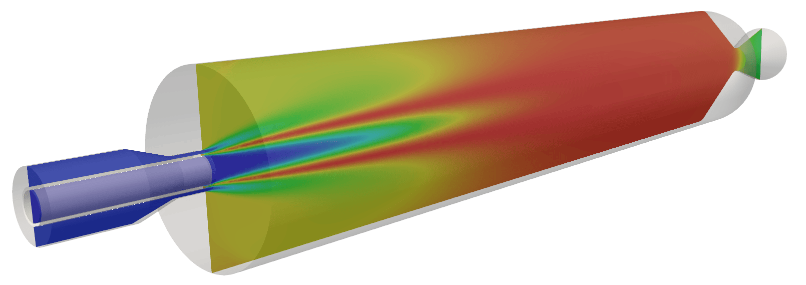Shown below are select plots of the solution variables.

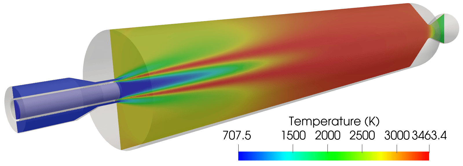
Contour plot of the temperature field for the RANS simulation.

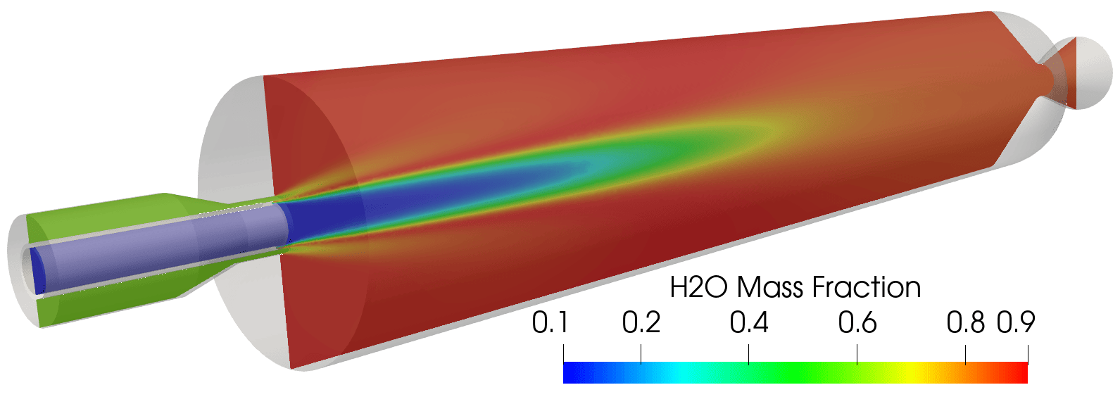
Contour plot of the H2O mass fraction field for the RANS simulation.

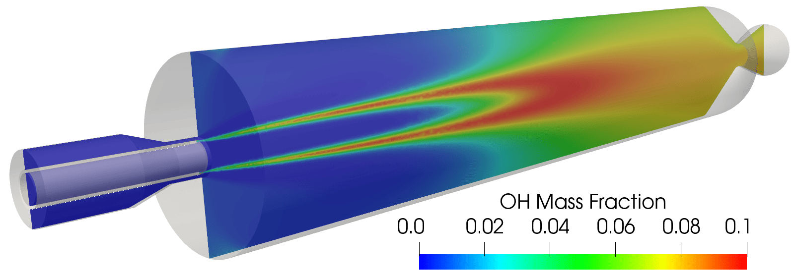
Contour plot of the OH mass fraction field for the RANS simulation.

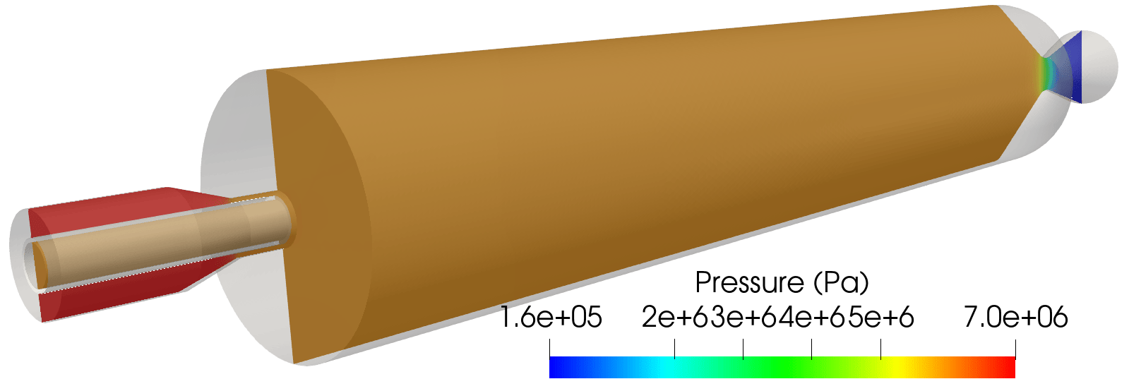
Contour plot of the pressure field for the RANS simulation. The compressible flamelet model captures realistic flow variations in the nozzle as can be seen by the pressure variation.

Run Control File Setup for DES Simulation

The run control file for the DES simulation is shown below.

Run control file for the DES case.

loadModule: compressible_flamelet_tf
{

// Grid file information.
grid_file_info: <file_type=VOG,Lref=1 m >

//*********************************
// P_chamber=5.4e+06 Pa

// Fuel Inlet: Temperature = 800 [K]
//        Massfraction-H2 = 0.4018
//        Massfraction-H2O = 0.5982

// Oxidizer Inlet: Temperature = 711 [K]
//        Massfraction-O2 = 0.9449
//        Massfraction-H2O = 0.0551
//*********************************

boundary_conditions:
<
Fuel_inlet=subsonicInlet(mdot=3.33111993e-02 kg/s,T=800 K,Z=1.0,C=0.5982,k=4.2,omega=12900.0),
Nozzle=noslip(adiabatic),
ChamberWalls=noslip(adiabatic),
Fuel_Walls=noslip(adiabatic),
Oxidizer_Walls=noslip(adiabatic),
Post_Tip=noslip(adiabatic),
Face_Plate=noslip(adiabatic),
Oxidizer_inlet=subsonicInlet(mdot=9.0447402E-02 kg/s,T=711 K,Z=0.0,C=0.0551,k=0.5,omega=37950.0),
Outlet=extrapolatedPressureOutlet,
Back_PieSlicet=symmetry,
Front_PieSlice=symmetry
>

// Initial condition.
initialCondition: <v=[0.0 m/s,0.0 m/s,0.0 m/s],p=5.4e+06 Pa,T=700.0 K,Z=0.0,C=0.0551,k=0.5,omega=37950.0>

// Flow properties
flowRegime: turbulent 
flowCompressibility: compressible

// Transport model set to 'module' since all properties gotten from flamelet table.
transport_model: module

// Time-integration parameters.
timeIntegrator: CN
CNBDFBlend: 0.9
timeStep: 3.0e-07
numTimeSteps: 50001
convergenceTolerance: 1.0e-12
maxIterationsPerTimeStep: 21

// InviscidFlux [FOU,SOU]
//inviscidFlux: SOU
//-------------------------------
inviscidFlux: SLAU
slau_mhat: 2         // 1 or 2 - default is 1
slau_reconstruct: 2  // 1 or 2 - default is 2
slau_pfactor: 0.0    // 1.0 or 0.0 - default is 1.0
//-------------------------------

turbulenceInviscidFlux: SOU
flameletInviscidFlux: SOU

// Gradient limiting.
limiter: NB

linearSolverTolerance: 1.0e-02
petscSolverName: GMRES
hypreSolverName: AMG
hypreStrongThreshold: 0.9

// Set the turn-over time scale used to normalize residual turn-over time values.
//diagnostics: <turnoverTimeScale=2.85e-03>

// Momentum equation (linearSolver[SGS],0.0<relaxationFactor<1.0)
momentumEquationOptions: <linearSolver=SGS,relaxationFactor=0.5,maxIterations=5>

// Pressure equation (linearSolver[SGS,PETSC,HYPRE],0.0<relaxationFactor<1.0)
pressureCorrectionEquationOptions: <linearSolver=HYPRE,relaxationFactor=0.5,maxIterations=20>
  pressureBasedMethod: SIMPLEC
  PclipMin: 20000.0
  PclipMax: 20000000.0

// Energy equation (linearSolver[SGS],0.0<relaxationFactor<1.0)
energyEquationOptions: <linearSolver=SGS,relaxationFactor=0.5,maxIterations=5,form=totalEnergy>
  TclipMin: 500.0
  TclipMax: 5000.0

// Turbulence equation
turbulenceEquationOptions: <model=menterSST2003,des=IDDES2012,linearSolver=SGS,relaxationFactor=0.5,maxIterations=5>
  turbulentPrandtlNumber: 0.7
  turbulentSchmidtNumber: 0.7

// Flamelet equation
flameletEquationOptions: <linearSolver=SGS,relaxationFactor=0.4,maxIterations=5>
  combustion: on

// Available combustion models. Model cost specified only if using PEC.
combustionModels:
<
  nonpremixed=flamelet(table="burke_fpvc_ideal_20200601.h5")
>

// Combustion model selection by region.
combustionModelRegions:
<
  regions=[
    inBox(p1=[-1.0e+30,-1.0e+30,-1.0e+30],p2=[1.0e+30,1.0e+30,1.0e+30],model=nonpremixed)
  ]
>

kFreestream: 4.2
omegaFreestream: 12900
eddyViscosityLimit: 10000

// Printing, plotting and restart parameters.
print_freq: 1000
plot_freq: 500
plot_modulo: 0
plot_output: ZZ,C,e,es,eos_dT,T0,E0,viscosityRatio
//plot_output_iteration: on
restart_freq: 1000
restart_modulo: 0

}

In the following, we briefly discuss some of the key choices made in setting the run control file parameters for the DES case.

1. While this case is being restarted from a RANS solution, note that we must still specify an initial condition in the run control file to circumvent Stream’s run control file consistency checking coding from returning an error. Upon restart, however, the values specified in the variable initialCondition will be ignored.

2. The DES simulation is a time-accurate simulation. As such, we have selected the blended Crank-Nicolson/BDF scheme with a blending factor of 0.9, which in our experience achieves time accuracy at a slightly larger time step than the BDF2 time-differencing scheme. Note that a relatively small time step of 2.0e-07 is still required for stability and time-accuracy purposes compared to the value chosen for the RANS simulation. Here we have used 21 iterations per time step, however, based on evaluation of the residual convergence in the run log file, one could probably use less and save CPU time.

3. For the inviscid fluxes, we have chosen the SLAU scheme, which is generally superior to SOU for compressible flows, and have also used second-order inviscid flux reconstruction for the turbulence and flamelet equations, in order to avoid the excess spatial dissipation one would get using the FOU scheme.

4. For the pressure-correction equation, one should always use the HYPRE linear solver. The parameters in the linear solver section apply only to the HYPRE solver and are not used by the SGS linear solver which is being employed here for the momentum, total energy and flamelet equations. Here we select the Algebraic Multi-Grid (AMG) solver, which is superior in general to the GMRES solver in HYPRE. We set the linear solver tolerance to a relatively high value of 1.0e-02 to avoid over solving the linear system for the pressure-correction equation. The hypreStrongThreshold parameter is set to a relatively high value (range 0-1,default is 0.5) to further minimize the work per linear solver iteration.

5. At the end of the run control file, for tutorial purposes, we show several variables (hypreSolverOutput, massTurnOverTimeOutput, residualMaximumOutput ) that can be used to monitor the health of the solution process. See the Stream users’ guide for details on these variables. For lengthy simulations (hundreds of thousands of timesteps) one should ensure that the values for these three diagnostic variables are off , in order to prevent debug files in the /debug directory from becoming excessively large (gigabytes).

Running the DES Simulation

In the tutorial main directory are three files that are required to run the RANS and DES cases.

• case.vog: the grid

• bc_temp.dat: a temperature profile along the upper wall of the combustor

• allstar_fpvc_ideal_20210203.h5: the flamelet table

Also in this directory is a sub-directory called des/ , which contains the run control file for this case.

To run the DES case, first copy the case.vog, bc_temp.dat, and allstar_fpvc_ideal_20210203.h5 files to the des/ directory. In addition, you will create a new directory in the des/ directory called restart/. This directory is where you will place a set of RANS restart files for the DES simulation to restart from. For this case, the RANS simulation was run to 10,000 timesteps and a set of restart files were written at the 10,000th timestep. Go to the rans/ directory and perform a copy like the one shown below.

cp restart/*10000* ../des/restart/

For this case, the grid has around 206,000 cells. Stream has parallel efficiency down to 5,000 cells per processor, so you will want to run using less than 40 processes for the value passed to the -np argument in the mpirun command shown below. Using fewer processes is fine and will only result in an increased time for the solution to be generated. Enter the des/ directory and execute the code using the following command.

• mpirun -np 40 <path_to_stream_exec> --scheduleoutput -q solution case 10000 >& run.log_10000 &

The DES case will run an additional number of timesteps from the restart as specified by the numTimeSteps variable in the case.vars file. The case will thus terminate at timestep 200,000. Restart checkpoint solutions will be written to the restart/ directory at the number of timesteps specified in the case.vars file for the restart_freq``variable. The addition of the integer argument ``10000 in the command above tells Stream to use the solution in the restart/ directory as the initial condition. In the command above, the file that the log information is redirected to is named run.log_10000. This suffix is used to differentiate the log file from other log files that are generated when a user is restarting cases. The suffix notation prevents log file information from previous simulations from being overwritten. The naming convention is not required, but is a good practice to follow when using Stream.