2D Shock Over A Sphere Tutorial

This tutorial will cover the basics of setting up and running the problem of a compressible flow with a shock wave passing over a stationary spherical object (sometimes called a ‘particle’ in this example). Additionally, a comparison of Stream results to experimental data will be presented.

In this problem a high pressure region is created upstream of a rigid particle (represented by the simulation boundary), and a shock wave forms and propagates across the domain and over the particle. There is experimental data for the force that a particle experiences under a flow condition like this one. This example will also include a comparison of the force that the simulated particle feels and the measured force from an experiment. The files that are needed to run this case can be extracted from a gzipped archive located here. The files will extract into a directory structure that mirrors this case’s location in the tutorials repository.

Geometry and Boundary Conditions

This case is set up as a axisymmetric shock tube problem. A high pressure region is created upstream of a rigid particle (represented by the simulation boundary), and a shock wave forms and propagates across the domain and over the particle. A subsonic inflow condition is set at the left boundary with conditions that match the high pressure state conditions to provide a driver of the shock front.

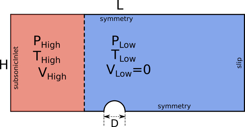
Geometry and boundary conditions for the supersonic flow over a sphere tutorial.

Grid

A triangular cell grid was generated using GMSH. This grid is a single-cell thick 3D mesh with an extrusion in the z-direction. The grid is comprised of 262,364 prismatic cells. An image of the region near the particle is shown below.

A close-up of the grid near the sphere.

To generate the mesh yourself, if you have GMSH installed, you can use the following .geo control file to generate the mesh.

GMSH .geo control file for the shock-over-sphere tutorial.

// This grid is drawn in millimeters
D = 80;
R = 0.5*D;

CX = 0.0;
CY = 0.0;

OuterCircleFactor = 2.5 ;
OuterDomainLeftFactor = 4; // How far to put left-most boundary
OuterDomainRightFactor = 6; // How far to put right-most boundary
OuterDomainUpperFactor = 4; // How far to put upper boundary
OuterRadius = OuterCircleFactor*D;

// Points for right-side patch around particle
Point(1) = {CX + R, CY, 0};
Point(2) = {CX + OuterRadius, CY, 0};

// Shared points between left and right patches
Point(3) = {CX, CY + OuterRadius, 0};
Point(4) = {CX, CY + R, 0};

// Points for left-side patch around particle
Point(5) = {CX - R, CY, 0};
Point(6) = {CX - OuterRadius, CY, 0};

Point(7) = {CX, CY, 0}; // Center point used to create a circle

// Points for rectangular outer domain
Point(8) = {CX + OuterDomainRightFactor*OuterRadius, CY, 0};
Point(9) = {CX + OuterDomainRightFactor*OuterRadius, CY + OuterDomainUpperFactor*OuterRadius, 0};
Point(10) = {CX - OuterDomainLeftFactor*OuterRadius, CY + OuterDomainUpperFactor*OuterRadius, 0};
Point(11) = {CX - OuterDomainLeftFactor*OuterRadius, CY, 0};

// Lines connecting particle patches
Line(1) = {1, 2};
Line(2) = {5, 6};
Line(3) = {3, 4};

// Particle boundary on right-side patch
Circle(4) = {1, 7, 4};
Circle(5) = {2, 7, 3};

// Particle boundary on left-side patch
Circle(6) = {5, 7, 4};
Circle(7) = {6, 7, 3};

// Lines connecting outer domain
Line(8) = {2, 8};
Line(9) = {8, 9};
Line(10) = {9, 10};
Line(11) = {10, 11};
Line(12) = {11, 6};


// Surface of right-side patch around particle
Curve Loop(1) = {1, 5, 3, -4};
Surface(1) = {1};

// Surface of left-side patch around particle
Curve Loop(2) = {2, 7, 3, -6};
Surface(2) = {2};

// Surface of domain around particle
Curve Loop(3) = {-5, 8, 9, 10, 11, 12, 7};
Plane Surface(3) = {3};

//---- Sizing field for uniform unstructured mesh near particle----
// Create a Distance field
DistanceField = 1;
Field[DistanceField] = Distance;
Field[DistanceField].SurfacesList = {1,2};
Field[DistanceField].Sampling = 200;

// Apply a Threshold field to control mesh size growth
ThresholdField = 2;
Field[ThresholdField] = Threshold;
Field[ThresholdField].IField = DistanceField; // Use the Distance field
Field[ThresholdField].LcMin = 0.8; // Minimum cell size
Field[ThresholdField].LcMax = 50; // Maximum cell size
Field[ThresholdField].DistMin = 10; // Distance for min cell size
Field[ThresholdField].DistMax = 400; // Distance for max cell size

// Set the Background Field
Background Field = ThresholdField;
//-------------------------------------------------------------------

// Generate a 2D mesh of the surface so that the mesh gets extruded too

Extrude {0, 0, -D} {
    Surface{1, 2, 3};
    Layers{1};
    Recombine;
}


Physical Surface("Inlet", 1) = {84};
Physical Surface("Particle", 2) = {55, 33};
Physical Surface("TopWall", 3) = {80};
Physical Surface("Symmetry", 4) = {43, 21, 72, 88};
Physical Surface("Outlet", 5) = {76};
Physical Surface("Front", 6) = {1, 2, 3};
Physical Surface("Back", 7) = {34, 56, 93};

Physical Volume(1) = {1,2,3};


Mesh 3;
Save "case.msh";

Once the mesh is generated, you can use the following Loci utility to create a vog file from the msh file.

msh2vog -mm case

This will create a case.vog file that can be used as the grid file for the simulation.

Run Control File Setup

The run control file for the simulation is shown below.

Run control file for the case.

{

// Grid file information
grid_file_info: <file_type=VOG, Lref=1 m>

gridCoordinates: axisymmetric

// Boundary conditions
boundary_conditions:
<
 Inlet=subsonicInlet(v=116.7856 m/s, T=347.8651 K),
 Particle=slip,
 TopWall=slip,
 Symmetry=symmetry,
 Outlet=extrapolatedPressureOutlet,
 Front=symmetry,
 Back=symmetry
>

// Initial condition
ql: <p=137357.5 Pa, T=347.8651 K, v=116.7856 m/s >
qr: <p=87500 Pa, T=305 K, v=0.0 m/s >
xmid: -0.06

// Flow properties
flowRegime: laminar
flowCompressibility: compressible

// Equation of state and transport properties.
chemistry_model: air_1s0r
transport_model: const_viscosity
mu: 1.0e-10
kcond: 1.0e-8

// Time-integration parameters
timeIntegrator: BDF2
timeStep: 5.0e-7
numTimeSteps: 2001
convergenceTolerance: 1.0e-12
maxIterationsPerTimeStep: 20

// Inviscid flux
inviscidFlux: SLAU

// Gradient limiting
limiter: venkatakrishnan

// Linear solver options
linearSolverTolerance: 1.0e-03
hypreSolverName: AMG
hypreStrongThreshold: 0.9

// Momentum equation
momentumEquationOptions: <linearSolver=SGS,relaxationFactor=0.7,maxIterations=5>

// Pressure correction equation
pressureCorrectionEquationOptions: <linearSolver=HYPRE,relaxationFactor=0.7,maxIterations=20>
  pressureBasedMethod: SIMPLEC

// Energy equation
energyEquationOptions: <linearSolver=SGS,relaxationFactor=0.7,maxIterations=5,form=temperature>

// Printing, plotting, and restart parameters
print_freq: 100
plot_freq: 100
plot_output: cfl
plot_modulo: 0
restart_freq: 2000
restart_modulo: 0

// Set debugging output
hypreSolverOutput: off
massTurnOverTimeOutput: off
residualMaximumOutput: off

}

In the following, we briefly discuss some of the key choices made in setting the run control file parameters for this case.

1. Due to the flow being supersonic with the prescence of strong shockwaves, the inviscidFlux variable is set to the SLAU2 scheme. The SLAU2 scheme is a second-order accurate flux-vector splitting scheme that is based on the Roe scheme, and it is designed to handle strong shockwaves.

2. The flow is essentially inviscid, so the viscosity and thermal conductivity are set to very low values. The flow is also compressible, so the flowCompressibility variable is set to compressible.

Running the Simulation

In the tutorial main directory are three files that are required to run the case.

• case.vog: the grid

• case.vars: the run control file

• air_1s0r: the .mdl file that contains the species definition for air that is used in this case.

The .mdl file is shown below for reference. More details about this file can be found in the Stream user guide.

The air_1s0r.mdl file.

// Model for Air as an ideal gas
species = {
  _Air   = < m=28.89, n=2.5, href=0, sref=0, Tref=298.0, Pref=10000.0, mf=1.0 > ;
} ;

reactions = {
} ;

For this case, the grid has around 260,000 cells. Stream has parallel efficiency down to 5,000 cells per processor, so you will want to run using less than 50 processes for the value passed to the -np argument in the mpirun command shown below. Using fewer processes is fine and will only result in an increased time for the solution to be generated. Execute the code using the following command.

mpirun -np 50 <path_to_stream_exec> --scheduleoutput -q solution case >& run.log_0 &

The case will run until the number of timesteps specified in the case.vars file is reached. Restart checkpoint solutions will be written to the restart/ directory at the number of timesteps specified in the case.vars file for the restart_freq variable.

Results

The metric used to compare the simulation results to the experimental data is the drag coefficient on the particle as a function of time. The stream-wise drag coefficient is just the force that the particle experiences along the horizontal axis divided by a parameter that is related to the downstream conditions and the cross-sectional area of the particle. The plot below shows the simulation results (in blue) capture the overall behavior of the experimental data. There is an under prediction of the peak force by about 5%.

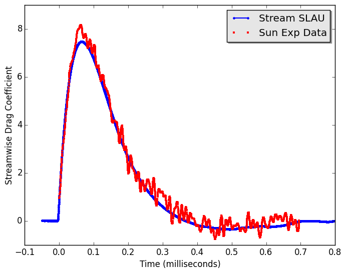
Comparison of the drag coefficient on the particle as a function of time between the simulation results and the experimental data.

The extract utility is used to view the results of a simulation. For this case we view the simulation at the 5,000th time step. In the run directory extract the solution using: extract -vtk case 5000 P v r t . This will generate a solution directory with files in the Paraview VTK format which can be opened by Paraview. The case name is case and the timestep is 5000, and the variables to extract are the pressure(P), velocity(v), density(r), and temperature(t). Below is a contour plot of the pressure field showing the primary and secondary reflected shock waves that occur during the passage of the initial planar shock wave.

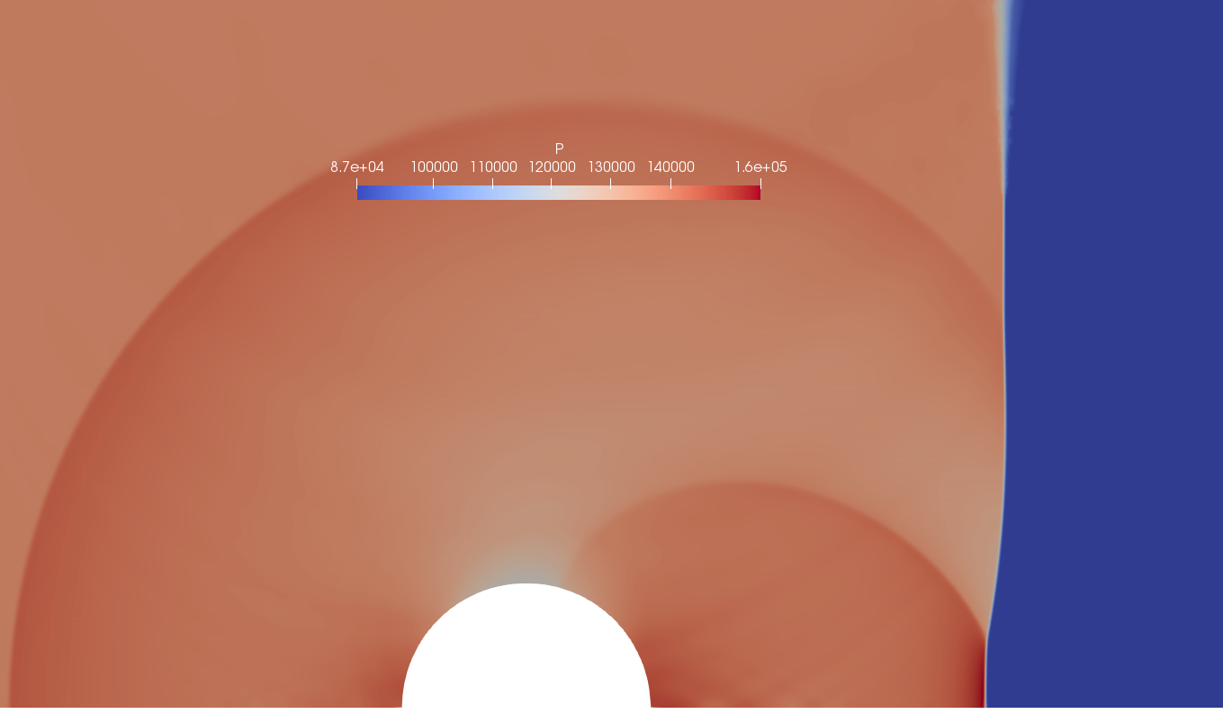
Contour plot of the pressure field at the 5,000th time step.