2D Supersonic Forward-Step Tutorial

This tutorial will cover the basics of setting up and running the problem of a supersonic flow passing over a forward-step. In this problem a supersonic flow of air moving at Mach 3 from left to right encounters a vertical step. The collision of the flow with this step produces a series of shock waves that propagate and reflect in the upper section. The files that are needed to run this case can be extracted from a gzipped archive located here. The files will extract into a directory structure that mirrors this case’s location in the tutorials repository.

Geometry and Boundary Conditions

The domain consists of a rectangular inlet with a 20 centimeter vertical jump placed 60 centimeters downstream of the inlet. The flow enters the domain on the left via a supersonic inlet boundary, and exits the domain through an extrapolated pressure outlet that is designed to handle supersonic flows.

Geometry and boundary conditions for the supersonic forward-step tutorial.

Grid

A triangular grid was generated using GMSH. This mesh is a single-cell extrusion into the z-direction. The grid is comprised of 194,914 prismatic cells. An image of the step region of the grid is shown below.

The grid in the vicinity of the vertical step. A uniform mesh spacing was used.

To generate the mesh yourself, if you have GMSH installed, you can use the following .geo control file to generate the mesh.

GMSH .geo control file for the forward-step tutorial.

// This GMSH file is drawn in units of meters

// Define points starting in lower left corner and going
// clockwise around the forward-step geometry
Point(1) = {0.0, 0.0, 0.0};
Point(2) = {0.0, 0.2, 0.0};
Point(3) = {0.0, 0.4, 0.0};
Point(4) = {0.0, 1.0, 0.0};
Point(5) = {0.6, 1.0, 0.0};
Point(6) = {1.0, 1.0, 0.0};
Point(7) = {3.0, 1.0, 0.0};
Point(8) = {3.0, 0.4, 0.0};
Point(9) = {3.0, 0.2, 0.0};
Point(10) = {1.0, 0.2, 0.0};
Point(11) = {0.6, 0.2, 0.0};
Point(12) = {0.6, 0.0, 0.0};


Point(13) = {0.6, 0.4, 0.0};
Point(14) = {1.0, 0.4, 0.0};

// Define lines that make up the domain
Line(1) = {1, 2};
Line(2) = {2, 3};
Line(3) = {3, 4};
Line(4) = {4, 5};
Line(5) = {5, 6};
Line(6) = {6, 7};
Line(7) = {7, 8};
Line(8) = {8,9};
Line(9) = {9, 10};
Line(10) = {10, 11};
Line(11) = {11, 12};
Line(12) = {12, 1};
Line(13) = {2, 11};
Line(14) = {11, 13};
Line(15) = {13, 5};
Line(16) = {3, 13};
Line(17) = {13, 14};
Line(18) = {14, 8};
Line(19) = {14, 6};
Line(20) = {10, 14};


// Define surfaces of the regions in the domain
Curve Loop(1) = {3, 4, -15, -16}; // Upstream, upper section
Surface(1) = {-1};

Curve Loop(2) = {2, 16, -14, -13}; // Upstream, middle section
Surface(2) = {-2};

Curve Loop(3) = {1, 13, 11, 12}; // Upstream, lower section
Surface(3) = {-3};

Curve Loop(4) = {19, 6, 7, -18}; // Outlet section, upper
Surface(4) = {-4};

Curve Loop(5) = {20, 18, 8, 9}; // Outlet section, lower
Surface(5) = {-5};

Curve Loop(6) = {15, 5, -19, -17}; // refinement section, upper
Surface(6) = {-6};

Curve Loop(7) = {14, 17, -20, 10}; // refinement section, lower
Surface(7) = {-7};

/*
//-----------Unstructured Mesh, refined corner------------------------
// Spacing numbers based on a cell-to-cell center spacing of 0.006m  in the bulk of the domain.
// A refinement near the top corner of the step is applied to bring the size down to 0.0015m

Field[1] = Distance;
Field[1].PointsList = {11};

Field[2] = Threshold;
Field[2].InField = 1;
Field[2].DistMax = 0.15;
Field[2].DistMin = 0.03;
Field[2].SizeMax = 0.006;
Field[2].SizeMin = 0.0015;
Background Field = 2;
//----------------------------------------------------
*/

//-----------Unstructured Mesh, uniform------------------------
// Spacing numbers based on a cell-to-cell center spacing of 0.00055m.

Field[1] = Distance;
Field[1].PointsList = {11};

Field[2] = Threshold;
Field[2].InField = 1;
Field[2].DistMax = 0.15;
Field[2].DistMin = 0.03;
Field[2].SizeMax = 0.0055;
Field[2].SizeMin = 0.0055;
Background Field = 2;
//----------------------------------------------------


width = -0.02;
Extrude {0, 0, width} {
Surface{1, 2, 3, 4, 5, 6, 7};
Layers{1};
Recombine;
}

Physical Surface("Inlet", 1) = {41, 63, 85};
Physical Surface("Walls", 2) = {73, 77, 161, 117, 103, 147, 37};
Physical Surface("Outlet", 3) = {99, 121};
Physical Surface("Symmetry", 4) = {1, 2, 3, 4, 5, 6, 7, 42, 64, 86, 152, 108, 130, 174 };

Physical Volume("internal", 1) = {1, 2, 3, 4, 5, 6, 7};

Mesh 3;
Save "case.msh";

Once the mesh is generated, you can use the following Loci utility to create a vog file from the msh file.

msh2vog -m case

This will create a case.vog file that can be used as the grid file for the simulation.

Run Control File Setup

The run control file for the simulation is shown below.

Run control file for the case.

{

// Grid file information
grid_file_info: <file_type=VOG, Lref=1m, twoDimensions>

// Boundary conditions
boundary_conditions: <
  Inlet=supersonicInlet(v=1029 m/s, p=101325 Pa, T=293 K),
  Outlet=extrapolatedPressureOutlet,
  Walls=symmetry,
  Symmetry=symmetry
>

// Initial conditions
initialCondition: <v=1029 m/s, p=101325 Pa, T=293.0 K>

// Flow properties
flowRegime: laminar
flowCompressibility: compressible

// Equation of state and transport properties
chemistry_model: air_1s0r
transport_model: const_viscosity
mu: 1.0e-10
kcond: 1.0e-10

// Time-stepping
timeIntegrator: BDF2
timeStep: 4.0e-6
numTimeSteps: 3001
convergenceTolerance: 1.0e-30
maxIterationsPerTimeStep: 30

// Inviscid flux
inviscidFlux: SLAU2

// Gradient limiting
limiter: mlp

// Linear solver options
linearSolverTolerance: 1.0e-03
hypreSolverName: AMG
hypreStrongThreshold: 0.9

// Diagnostics variables
//  turnoverTimeScale: used to normalize residual turn-over time (TT) values
diagnostics: <turnoverTimeScale=2.91e-03>

// Momentum equation
momentumEquationOptions: <linearSolver=SGS,relaxationFactor=0.7,maxIterations=5>

// Pressure correction equation
pressureCorrectionEquationOptions: <linearSolver=HYPRE,relaxationFactor=0.5,maxIterations=20>
  pressureBasedMethod: SIMPLEC
  PclipMin: 100.0

// Energy equation
energyEquationOptions: <linearSolver=SGS,relaxationFactor=0.7,maxIterations=5,form=totalEnthalpy>
  TclipMin: 100.0

// Printing, plotting, and restart parameters
print_freq: 1000
plot_freq: 100
plot_modulo: 0
plot_output: h,cfl
restart_freq: 1000
restart_modulo: 0

}

In the following, we briefly discuss some of the key choices made in setting the run control file parameters for this case.

1. Due to the flow being supersonic with the presence of strong shockwaves, the inviscidFlux variable is set to the SLAU2 scheme. The SLAU2 scheme is a second-order accurate flux-vector splitting scheme that is based on the Roe scheme, and it is designed to handle strong shockwaves.

2. The flow is inviscid, so the viscosity and thermal conductivity are set to very low values. The flow is also compressible, so the flowCompressibility variable is set to compressible.

3. For this grid geometry and flow conditions, solution convergence cannot be obtained using the venkatakrishnan limiter. Here we set the limiter variable to mlp which is more robust than the standard venkatakrishnan limiter for flows with shockwaves on unstructured meshes.

4. The timestep for this case is influenced by the maximum CFL number in the flow field. Since Stream uses implicit time integration, the code is able to run at CFL values larger than one, however there is generally a maximum CFL that is problem-dependent. For this case, the largest timestep that could be run was 4.0e-6, which results in a maximum CFL in the domain of about 4.

Running the Simulation

In the tutorial main directory are three files that are required to run the case.

• case.vog: the grid

• case.vars: the run control file

• air_1s0r: the .mdl file that contains the species definition for air that is used in this case.

The .mdl file is shown below for reference. More details about this file can be found in the Stream user guide.

The air_1s0r.mdl file.

// Model for Air as an ideal gas
species = {
  _Air   = < m=28.89, n=2.5, href=0, sref=0, Tref=298.0, Pref=10000.0, mf=1.0 > ;
} ;

reactions = {
} ;

For this case, the grid has around 195,000 cells. Stream has parallel efficiency down to 5,000 cells per processor, so you will want to run on no more than 40 processes for the value passed to the -np argument in the mpirun command shown below. Using fewer processes is fine and will only result in an increased time for the solution to be generated. Execute the code using the following command.

mpirun -np 40 <path_to_stream_exec> --scheduleoutput -q solution case >& run.log_0 &

The case will run until the number of timesteps specified in the case.vars file is reached. Restart checkpoint solutions will be written to the restart/ directory at the number of timesteps specified in the case.vars file for the restart_freq variable.

Results

The extract utility is used to view the results of a simulation. For this case we view the simulation at time step 2,000. In the run directory extract the solution using: extract -vtk forwardStep 2000 P v r t m a . This will generate a solution directory with files in the Paraview VTK format which can be opened by Paraview. The case name is case and the timestep is 2000, and the variables to extract are the pressure(P), velocity(v), density(r), temperature(t), mach number(m), and speed of sound(a). Below are contour plots of the pressure and mach number fields showing the bow shock on the left and the reflected shocks in the region past the step.

Contour plot of the pressure in the flow field at timestep 2,000 (physical time of 8.0e-3 seconds).

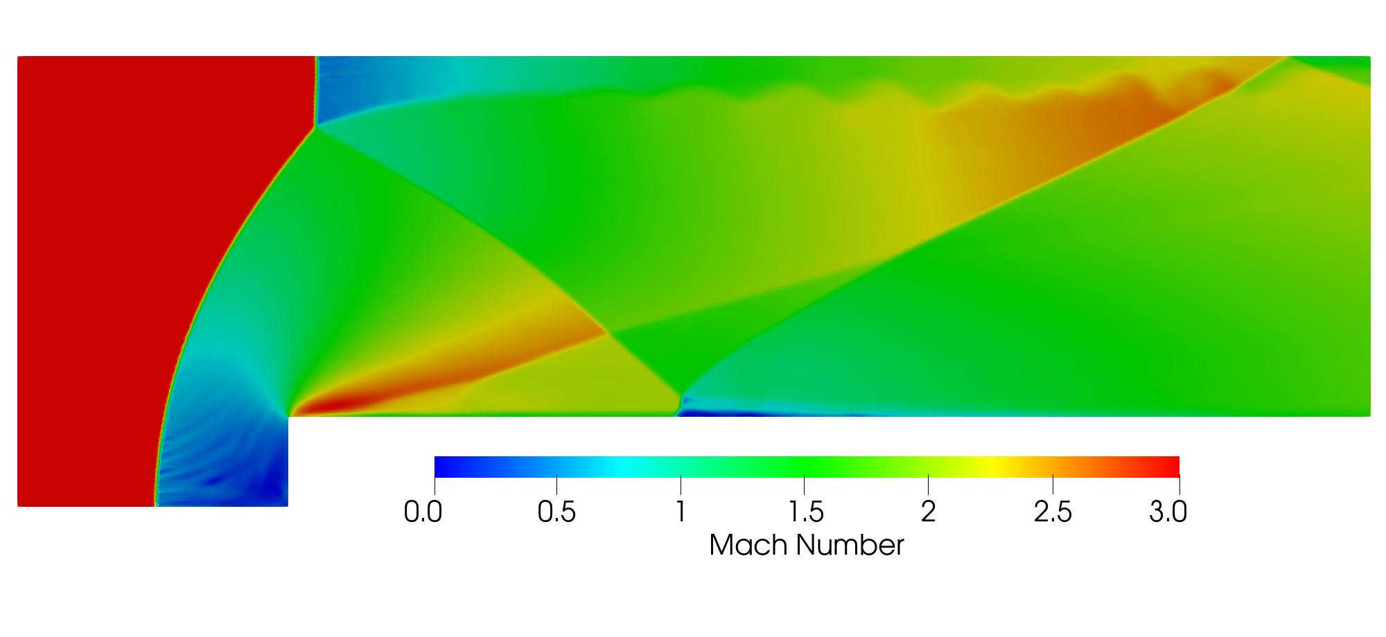
Contour plot of the mach number in the flow field at timestep 2,000 (physical time of 8.0e-3 seconds).

Alternative Refined Grid Simulation

The grid used above has a uniform mesh. For this case, in order to reproduce some of the visual results that are seen in literature, a more refined mesh is needed in the top corner region of the step. This prevents the formation of a Mach stem along the bottom surface. To generate the more refined mesh and run the refined case yourself, you can do the following:

1. Uncomment the lines in the .geo file for the section titled Unstructured Mesh, refined corner. The .geo uses standard C-style comments, so you will simply just remove the /* ... */ comments around the refined corner section and add a pair of /* ... */ comments around the Unstructured Mesh, uniform section. Then you can re-run the .geo file in GMSH to generate the .msh mesh, and follow the steps that are outlined in the grid section above to generate the .vog file.

2. The mesh with the more finely resolved region near the corner requires a smaller timestep for stability, and therefore you will need to lower the dt variable in the run control file to a value of 1.0e-6, and set the value for the numTimeSteps variable to 12000. With this lower timestep, a value of 21 for the maxIterationsPerTimeStep variable is sufficient for convergence within each timestep.

The refined mesh will look like the following:

The refined grid in the vicinity of the vertical step.

Contour plot of the pressure in the flow field at timestep 8,000 (physical time of 8.0e-3 seconds).