2D NASA Backward-Facing Step Tutorial

This tutorial will cover the basics of setting up and running the common fluid problem of the flow over a backward step. Additionally, a comparison of Stream results will be presented.

The backward step problem is commonly used to validate simulation codes’ turbulence models. It provides a case that is easy to setup and run, and there is quality empirical data available about the flow. In the backward facing step problem, a turbulent boundary layer encounters a sudden drop which causes a separation of the flow. The flow recovers some distance downstream of the drop. For a step height of H, the Reynolds number for this validation case is 36,000. This example is modeled after the data generated & provided by NASA Langley’s Turbulence Modeling Resource web page. The files that are needed to run this case can be extracted from a gzipped archive located here. The files will extract into a directory structure that mirrors this case’s location in the tutorials repository.

Geometry and Boundary Conditions

A subsonic flow of air at Mach 0.3 is directed over a step. The flow is directed from left to right, and a recirculation zone is formed in the region downstream of the step.

Geometry and boundary conditions for the NASA backward-facing step tutorial.

Grid

The grid for the case is the grid type 0 from the turbulence modeling website, a plot3D geometry file was downloaded and converted to the vog format using plot3d2vog utility. The grid is comprised of 1,277,952 hexahedral cells. The grid is a single cell thickness in the z-direction.

The structured grid in the region of the step.

Run Control File Setup

The run control file for the simulation is shown below.

Run control file for the case.

{

// Grid file information
grid_file_info: <file_type=VOG, Lref=1m, pieSlice>

boundary_conditions: <
 BC_1=noslip(adiabatic),                    //Upstream Bottom Wall
 BC_2=noslip(adiabatic),                    // Top Wall
 BC_3=subsonicInlet(T=537.0 R, v=41.7096 m/s, k=0.00097, omega=5091),  //Inlet
 BC_5=symmetry,                             //Backwall
 BC_6=symmetry,                             // Frontwall
 BC_13=noslip(adiabatic),                   // Bottom of Downstream section
 BC_15=noslip(adiabatic),                   // Vertical Step Face
 BC_22=fixedPressureOutlet(pMean=1.0 atm)  // Outlet
>

// Initial conditions
initialCondition: <p=1 atm, T=537.0 R, v=41.7096 m/s, k=0.00097, omega=5091>

// Flow properties
flowRegime: turbulent
flowCompressibility: compressible

// Equation of state and transport properties
chemistry_model: air_1s0r
transport_model: const_viscosity
mu: 2.498e-5
kcond: 4.175e-2

// Time-stepping
timeIntegrator: BDF
timeStep: 5e-3
numTimeSteps: 10001
convergenceTolerance: 1.0e-30
maxIterationsPerTimeStep: 15

// Inviscid flux options
inviscidFlux: SOU
turbulenceInviscidFlux: SOU

// Gradient limiting
limiter: venkatakrishnan

// Linear solver options
linearSolverTolerance: 1.0e-02
hypreSolverName: GMRES
hypreStrongThreshold: 0.9

// Diagnostics variables
//  turnoverTimeScale: used to normalize residual turn-over time (TT) values
diagnostics: <turnoverTimeScale=1.03e-01>

// Momentum equation
momentumEquationOptions: <linearSolver=SGS,relaxationFactor=0.5,maxIterations=5>

// Pressure equation
pressureCorrectionEquationOptions: <linearSolver=HYPRE,relaxationFactor=0.1,maxIterations=50>
  pressureBasedMethod: SIMPLEC

// Energy equation
energyEquationOptions: <linearSolver=SGS,relaxationFactor=0.5,maxIterations=5,form=temperature>

// Turbulence equation
turbulenceEquationOptions: <model=menterSST2003,linearSolver=SGS,relaxationFactor=0.5,maxIterations=5>

kFreestream: 0.00097
omegaFreestream: 5091
eddyViscosityLimit: 10000

// Printing, plotting, and restart parameters
print_freq: 500
plot_freq: 2500
plot_output: k, omega, a, pResidualTT, laminarViscosity, viscosityRatio
plot_modulo: 0
restart_freq: 2500
restart_modulo: 0

}

Running the Simulation

In the tutorial main directory are three files that are required to run the case.

• case.vog: the grid

• case.vars: the run control file

• air_1s0r: the .mdl file that contains the species definition for air that is used in this case.

The .mdl file is shown below for reference. More details about this file can be found in the Stream user guide.

The air_1s0r.mdl file.

// Model for Air as an ideal gas
species = {
  _Air   = < m=28.89, n=2.5, href=0, sref=0, Tref=298.0, Pref=10000.0, mf=1.0 > ;
} ;

reactions = {
} ;

For this case, the grid has around 1,300,000 cells. Stream has parallel efficiency down to 5,000 cells per processor, so you will want to run using less than 260 processes for the value passed to the -np argument in the mpirun command shown below. Using fewer processes is fine and will only result in an increased time for the solution to be generated. Execute the code using the following command.

mpirun -np 260 <path_to_stream_exec> --scheduleoutput -q solution case >& run.log_0 &

The case will run until the number of timesteps specified in the case.vars file is reached. Restart checkpoint solutions will be written to the restart/ directory at the number of timesteps specified in the case.vars file for the restart_freq variable.

Results

The results from the Stream simulation of the backward facing step flow problem are compared to experimental data for the problem as well as simulation data from a different NASA CFD code (CFL3D). Four locations along the stream-wise (horizontal) direction are sampled and data collected along the vertical direction.

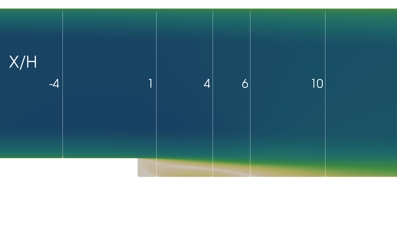
Locations for sampling data for comparison to experimental and other simulation data.

In the image above, the X-coordinate stations where the flow is sampled along the vertical direction to obtain data to compare to experimental results. X=0 is located at the step.

A note about the data presented below, the left plot appears to not have data from Stream, but all data sets are presented. They overlap considerably in the velocity space (circle data points can be seen near the top of the plot). The discrepancy between CFL3D and Stream is somewhat more pronounced for the stress plot.

Comparison plot of the velocity profile at the four locations.

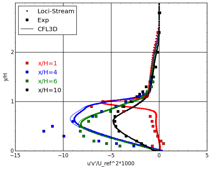
Comparison plot of the stress profile at the four locations.

The extract utility is used to view the results of a simulation. For this case we view the simulation at the 10,000th time step. In the run directory extract the solution using: extract -vtk case 10000 P v . This will generate a solution directory with files in the Paraview VTK format which can be opened by Paraview. The case name is case and the timestep is 10000, and the variables to extract are the pressure(P) and velocity(v). Below is shown a contour plot of the magnitude of the velocity field that was created using Paraview.

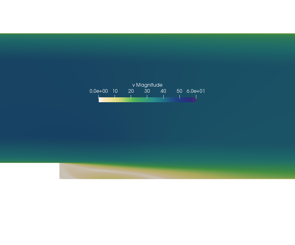
Contour plot of the magnitude of the velocity magnitude field at the 10,000th time step.