2D Karman Vortex Tutorial
This tutorial will cover the basics of setting up and running the fluid problem of the flow past a sphere to generate a Kármán vortex street. The Kármán vortex street is the laminar oscillation of vortices that is shown in the animation below. It is a fluid instability problem for viscous flows. The Strouhal number is a non-dimensional number that is used in when considering vortex induced vibrations. A Strouhal number of 0.2 corresponds to the formation of the steady shedding of vortices from the cylinder. This example sets up a flow condition such that the Strouhal number is around 0.2. The flow is incompressible, viscous, and bounded within a sealed 2D box. A steady uniform flow moves across the cylinder. The files that are needed to run this case can be extracted from a gzipped archive located here. The files will extract into a directory structure that mirrors this case’s location in the tutorials repository.
Geometry and Boundary Conditions
The domain is rectangular with an incompressible flow coming from the left boundary and flowing to the right and out of a fixed pressure boundary.

Geometry and boundary conditions for the Kármán vortex tutorial.
A Strouhal number around 0.2 is desired for this case to generate the Kármán vortex street. The Strouhal number is defined as:
- where:
\(St\) is the Strouhal number
\(f\) is the frequency of the vortex shedding
\(L\) is the characteristic length of the cylinder
\(U\) is the free stream velocity
A Reynolds number between 100 to 10,000 can showcase the instability phenomenon . The Reynolds number is defined as:
- where:
\(Re\) is the Reynolds number
\(U\) is the free stream velocity
\(L\) is the characteristic length of the cylinder
\(\mu\) is the dynamic viscosity of the fluid
\(\rho\) is the density of the fluid
- For this case, the setup was constructed by assuming the following values:
\(St\) = 0.2
\(Re\) = 5000
\(L\) = 0.01 m
\(\mu\) = 0.001 Pa*s
\(\rho\) = 1000 \(kg/m^3\)
With these assumptions the shedding frequency is expected to be around 10 Hz and the free stream velocity is around 0.5 m/s.
Grid
A mixed quadrilateral cell grid was first generated using GMSH . This was then extruded into a single-cell thick grid in the z-direction. The grid is comprised of 49,500 hexahedral cells. A few images of select regions of the grid are shown below.

The entire grid for the Kármán vortex tutorial.

Zoomed in view of the grid near the cylinder.
To generate the mesh yourself if you have GMSH installed. The following .geo control file can be loaded into GMSH to
generate the mesh used in this tutorial.
.geo control file for the tutorial.// This grid is drawn in units of meters
d = 0.1; // Diameter of the particle
offset = 2*d; // Distance away from particle where structured circular grid extends to
upstream_offset = 5*d ;
downstream_offset = 15*d;
vertical_offset = 6*d;
wake_factor = 1.25; // How much higher to place the downstream points to create a growing wake region in the mesh
theta = 45 * Pi / 180.0 ;
alpha = Cos(theta);
// Center of particle point
Point(1) = {0, 0, 0};
// Define points on the surface of the particle
Point(2) = {d/2*alpha, d/2*alpha, 0};
Point(3) = {-d/2*alpha, d/2*alpha, 0};
Point(4) = {-d/2*alpha, -d/2*alpha, 0};
Point(5) = {d/2*alpha, -d/2*alpha, 0};
// Define points for circular grid around particle
Point(6) = {offset*alpha, offset*alpha, 0};
Point(7) = {-offset*alpha, offset*alpha, 0};
Point(8) = {-offset*alpha, -offset*alpha, 0};
Point(9) = {offset*alpha, -offset*alpha, 0};
// Define corner points for outer boundary
Point(10) = {-upstream_offset*alpha, -vertical_offset*alpha, 0};
Point(11) = {-upstream_offset*alpha, vertical_offset*alpha, 0};
Point(12) = {downstream_offset*alpha, vertical_offset*alpha, 0};
Point(13) = {downstream_offset*alpha, -vertical_offset*alpha, 0};
// Define points on the horizontal outer boundaries
Point(14) = {offset*alpha, vertical_offset*alpha, 0};
Point(15) = {-offset*alpha, -vertical_offset*alpha, 0};
Point(16) = {-offset*alpha, vertical_offset*alpha, 0};
Point(17) = {offset*alpha, -vertical_offset*alpha, 0};
// Define points on the vertical outer boundaries
Point(18) = {-upstream_offset*alpha, -offset*alpha, 0};
Point(19) = {-upstream_offset*alpha, offset*alpha, 0};
Point(20) = {downstream_offset*alpha, wake_factor*offset*alpha, 0}; // Make this point a little higher to capture wake region
Point(21) = {downstream_offset*alpha, -wake_factor*offset*alpha, 0}; // Make point a little lower to capture wake region
// Define circle of the particle
Circle(1) = {4, 1, 3};
Circle(2) = {3, 1, 2};
Circle(3) = {2, 1, 5};
Circle(4) = {5, 1, 4};
// Define circle around circular offset around particle
Circle(5) = {8, 1, 7};
Circle(6) = {7, 1, 6};
Circle(7) = {6, 1, 9};
Circle(8) = {9, 1, 8};
// Define outer boundary
Line(9) = {10, 18};
Line(10) = {18,19};
Line(11) = {19, 11};
Line(12) = {11,16};
Line(13) = {16,14};
Line(14) = {14,12};
Line(15) = {12,20};
Line(16) = {20,21};
Line(17) = {21,13};
Line(18) = {13,17};
Line(19) = {17,15};
Line(20) = {15,10};
// Define Lines around particle
Line(21) = {3,7};
Line(22) = {2,6};
Line(23) = {4,8};
Line(24) = {5,9};
// Define lines moving from particle to boundary
Line(25) = {8,18};
Line(26) = {7,19};
Line(27) = {7,16};
Line(28) = {6,14};
Line(29) = {8,15};
Line(30) = {9,17};
Line(31) = {6,20};
Line(32) = {9,21};
// Define Surfaces
Curve Loop(1) = {23, 5, -21, -1};
Plane Surface(1) = {1};
Curve Loop(2) = {21, 6, -22, -2};
Plane Surface(2) = {2};
Curve Loop(3) = {22, 7, -24, -3};
Plane Surface(3) = {3};
Curve Loop(4) = {4, 23, -8, -24};
Plane Surface(4) = {4};
Curve Loop(5) = {25, 10, -26, -5};
Plane Surface(5) = {5};
Curve Loop(6) = {26, 11, 12, -27};
Plane Surface(6) = {6};
Curve Loop(7) = {27, 13, -28, -6};
Plane Surface(7) = {7};
Curve Loop(8) = {28, 14, 15, -31};
Plane Surface(8) = {8};
Curve Loop(9) = {7, 32, -16, -31};
Plane Surface(9) = {9};
Curve Loop(10) = {32, 17, 18, -30};
Plane Surface(10) = {10};
Curve Loop(11) = {30, 19, -29, -8};
Plane Surface(11) = {11};
Curve Loop(12) = {29, 20, 9, -25};
Plane Surface(12) = {12};
// Define Transfinite edge spacings
// Vertical far boundaries
Transfinite Curve {11, 27, 28, 15, 9, 29, 30, 17} = 31 Using Progression 1;
// Upstream far horizontal boundaries
Transfinite Curve {20, 25, 26, 12} = 31 Using Progression 1;
// Downstream far horizontal boundaries
Transfinite Curve {14, 31, 32, -18} = 61 Using Progression 1.05;
// Refined region, upstream, vertical boundaries
Transfinite Curve {10, 5, 1} = 31 Using Progression 1;
// Refined region, downstream, vertical boundaries
Transfinite Curve {3, 7, 16} = 121 Using Progression 1;
// Refined region, symmetric vertical region, horizontal boundaries
// (boundaries above and below the particle in the refinement region)
Transfinite Curve {19, 8, 4, 2, 6, 13} = 61 Using Progression 1;
// Boundary layer boundaries that intersect particle surface
Transfinite Curve {-21, -22, -24, -23} = 121 Using Progression 0.95;
Transfinite Surface "*";
Recombine Surface "*";
extrude_width = -0.5*d;
Extrude {0, 0, extrude_width} {
Surface{1, 2, 3, 4, 5, 6, 7, 8, 9, 10, 11, 12};
Layers{1};
Recombine;
}
Physical Surface("Inlet", 1) = {155, 133, 291};
Physical Surface("Particle", 2) = {53, 75, 97, 107};
Physical Surface("Walls", 3) = {159, 177, 199, 287, 265, 247};
Physical Surface("Symmetry", 4) = {1,2,3,4,5,6,7,8,9,10,11,12,54,98,296,142,164,274,120,76,186,252,230,208};
Physical Surface("Outlet", 5) = {243,225,203};
Physical Volume(1) = {1,2,3,4,5,6,7,8,9,10,11,12};
Mesh 3;
Save "case.msh";
Once the mesh is generated, you can use the following Loci utility to create a vog file from the msh file.
msh2vog -m case
This will create a case.vog file that can be used as the grid file for the simulation.
Run Control File Setup
The run control file for the simulation is shown below.
{
// Grid file information
grid_file_info: <file_type=VOG, Lref=1m, pieSlice>

boundary_conditions: <
 Inlet=incompressibleInlet(v=0.5 m/s),
 Outlet=fixedPressureOutlet(p=1 Pa),
 Walls=slip(),
 Particle=noslip(),
 Symmetry=symmetry()
>

// Initial conditions
initialCondition: <rho=1000, p=1 Pa, v=0.0 m/s>

// Flow properties
flowRegime: laminar
flowCompressibility: incompressible

// Equation of state and transport properties
transport_model: const_viscosity
mu: 1e-3

// Time-stepping
timeIntegrator: BDF2
timeStep: 1.0e-3
numTimeSteps: 5001
convergenceTolerance: 1.0e-30
maxIterationsPerTimeStep: 15

// Inviscid flux
inviscidFlux: SOU

// Gradient limiting
limiter: venkatakrishnan

// Linear solver options
linearSolverTolerance: 5.0e-02
hypreSolverName: AMG

// Set the turn-over time scale used to normalize residual turn-over time values.
diagnostics: <turnoverTimeScale=2e-1>

// Momentum equation
momentumEquationOptions: <linearSolver=SGS,relaxationFactor=0.7,maxIterations=3>

// Pressure equation
pressureCorrectionEquationOptions: <linearSolver=HYPRE,relaxationFactor=0.5,maxIterations=20>
  pressureBasedMethod: SIMPLEC


// Printing, plotting, and restart parameters
print_freq: 20
plot_freq: 25
plot_modulo: 0
plot_output: pResidualTT
restart_freq: 250
restart_modulo: 0

}
Running the Simulation
In the tutorial main directory are three files that are required to run the case.
case.vog: the grid
case.vars: the run control file
For this case, the grid has around 103,000 cells. Stream has parallel efficiency down to 5,000 cells per processor, so you will
want to run using less than 20 processes for the value passed to the -np argument in the mpirun command shown below. Using fewer
processes is fine and will only result in an increased time for the solution to be generated. Execute the code using the following command.
mpirun -np 20 <path_to_stream_exec> --scheduleoutput -q solution case >& run.log_0 &
The case will run until the number of timesteps specified in the case.vars file is reached. Restart checkpoint solutions will be
written to the restart/ directory at the number of timesteps specified in the case.vars file for the restart_freq variable.
Results
The extract utility is used to view the results of a simulation. The simulation is viewed at the 500th time step. In the run directory extract the solution
using: extract -vtk case 500 P v . This will generate a solution directory with files in the Paraview VTK format which can be opened by Paraview. The case
name is case and the timestep is 500, and the variables to extract are the pressure(P) and velocity(v). Below is a contour plot of the vorticity of the
flow that was created using Paraview.
For users of Paraview who may want to reproduce this image, just apply the GradientOfUnstructuredDataSet filter (Filter->GradientOfUnstructuredDataSet), enable
the advanced options on the filter (click the gear icon at the top right, and check the compute vorticity box).
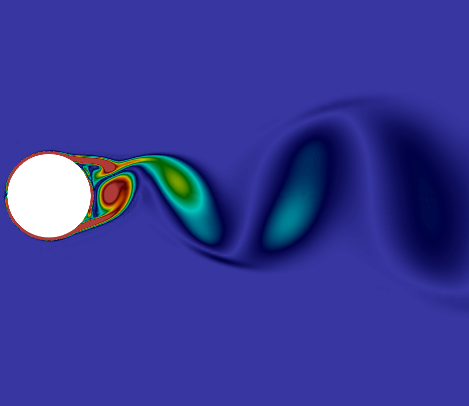
Contour plot of the vorticity of the flow past a cylinder at the 500th time step.